Tips and Tricks to Know in R

This is a set of tips and tricks to know when coding in R which aren’t for beginners but not as advanced as Hadley Wickham advance-R.

The idea is to compile the best practice in R which had increased my productivity in the last years and share them.

When working with Rstudio, one project = one folder

Project could be found in file -> New Project…

This is especially a good advice if you work on different projects or are used to have multiple sessions of R open at the same time.

It allows to fastly close and open a project, as the session is saved, including the tab of your session and the data in your memory.

The only thing to take care is to have a light amount of data in memory. Otherwise, the project could take a while to close. If it becomes problematic, there is an option in Tools>global options>untick “always save history” to change that.

Personally, I like to organise my project in the following directory structure: Project

– – R

– – doc

– – data

– – plot

– – output

It is similar to the folder structure used when creating a package, with doc and output in addition.

Style your code

As R is a case sensitive language, it is very important to define a style property that you keep across all your programs.

I am a big fan of google style (10 min) when coding in R.

The most important rules:

• Place spaces around all binary operators (=, +, -, <-, etc.).
• Exception: Spaces around ='s are optional when passing parameters in a function call.
• Do not place a space before a comma, but always place one after a comma.
• The preferred form for variable names is all lower case letters and words separated with dots (variable.name).
• Function names have initial capital letters and no dots (FunctionName).

Use data.table

The data.table is the package which make me consider R as a software which could be used as equal to SAS (at least in marketing studies).

The concepts could be tough at the beginning, but after a few time of practice, your productivity is multiplied.

The data.table allows, among others:

• Fast import of csv.
• Fast merging through indexation.
• Fast variable modification.
• Fast summarisation of data.
• Fast ranking process.

The only function needed to make this package the core data management in R is a version of sqlQuery of the RODBC package which query database directly into data.table.

Some exemple of utilisation: For more, read the introduction: (10 min here: data.table intro)

# conversion to data.table of the diamond data set:
diamonds.dt <- data.table(diamonds)

# variable of interest: numeric variables to compile
var.of.interest <- c("carat", "depth", "price", "x", "y", "z")

# mean of the variable of interest by cut:
diamonds.dt[, lapply(.SD, mean), by = cut, .SD = var.of.interest]

##          cut     carat    depth    price        x        y        z
## 1:     Ideal 0.7028370 61.70940 3457.542 5.507451 5.520080 3.401448
## 2:   Premium 0.8919549 61.26467 4584.258 5.973887 5.944879 3.647124
## 3:      Good 0.8491847 62.36588 3928.864 5.838785 5.850744 3.639507
## 4: Very Good 0.8063814 61.81828 3981.760 5.740696 5.770026 3.559801
## 5:      Fair 1.0461366 64.04168 4358.758 6.246894 6.182652 3.982770

# median and count of the variable of interest by cut:
median.unique <- function(x) quantile(x, probs = 0.5)
diamonds.dt[, c(lapply(.SD, median.unique), count = .N), by = cut, .SD = var.of.interest]

##          cut carat depth  price     x    y    z     N
## 1:     Ideal  0.54  61.8 1810.0 5.250 5.26 3.23 21551
## 2:   Premium  0.86  61.4 3185.0 6.110 6.06 3.72 13791
## 3:      Good  0.82  63.4 3050.5 5.980 5.99 3.70  4906
## 4: Very Good  0.71  62.1 2648.0 5.740 5.77 3.56 12082
## 5:      Fair  1.00  65.0 3282.0 6.175 6.10 3.97  1610

# count of all the diamonds away from the mean of more than to sd:(number of
# potential outliers).
away.sd <- function(x) sum(abs(x - mean(x)) > 2 * sd(x))
diamonds.dt[, c(lapply(.SD, away.sd), count = .N), by = cut, .SD = var.of.interest]

##          cut carat depth price   x   y   z     N
## 1:     Ideal  1020   855  1390 711 656 717 21551
## 2:   Premium   831   564   942 253 123 240 13791
## 3:      Good   226   402   305 159 168 164  4906
## 4: Very Good   532   499   762 422 402 249 12082
## 5:      Fair    61   115   106  77  76  76  1610

# even better, the percentage formatted table:
format2 <- function(x) lapply(x, function(x) sprintf("%1.3f%%", x))
away.sd2 <- function(x) format2(sum(abs(x - mean(x)) > 2 * sd(x))/length(x))
diamonds.dt[, c(lapply(.SD, away.sd2), count = .N), by = cut, .SD = var.of.interest]

##          cut  carat  depth  price      x      y      z     N
## 1:     Ideal 0.047% 0.040% 0.064% 0.033% 0.030% 0.033% 21551
## 2:   Premium 0.060% 0.041% 0.068% 0.018% 0.009% 0.017% 13791
## 3:      Good 0.046% 0.082% 0.062% 0.032% 0.034% 0.033%  4906
## 4: Very Good 0.044% 0.041% 0.063% 0.035% 0.033% 0.021% 12082
## 5:      Fair 0.038% 0.071% 0.066% 0.048% 0.047% 0.047%  1610

This is only a glipse of what could be done with the data.table packages. All I used to do in SQL before, I now do it with data.table.

Mastering ggplot2

A good way to aprehend a set of data is to use data visualisation. The ggplot2 package allows, when mastered, to do highly customised graph. Even XKCD-like ones (In this case, replace perl by ggplot2).

The official documentation is well made, but for beginners, this excellent blog is more appropriate.

# exemple, for the diamonds data set:
p1 <- ggplot(aes(x = carat, y = price, colour = cut), data = diamonds.dt) +
  geom_point(colour = "black", size = 3) +  geom_point()

p2 <- ggplot(aes(x = carat, y = price, colour = clarity), data = diamonds.dt) +
  geom_point(colour = "black", size = 3) +  geom_point()

grid.arrange(p1, p2, nrow = 1, ncol = 2)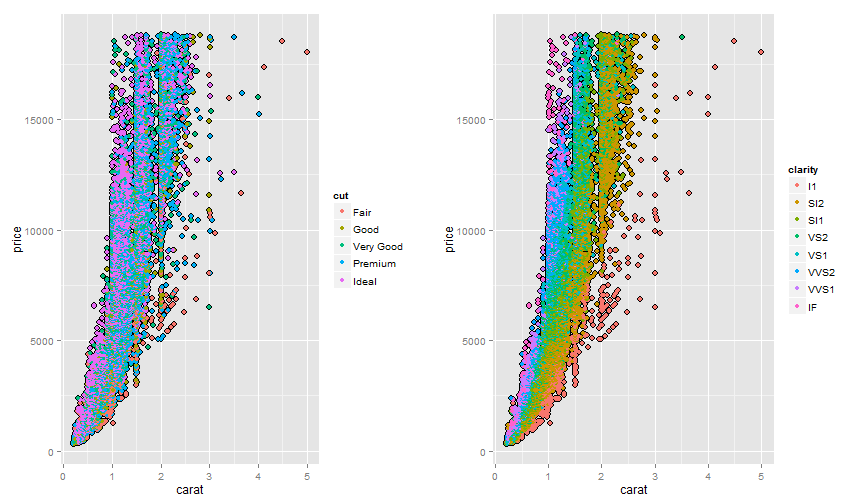

A few concepts are good to handle:

• A ggplot2 object could be stored.
• Customise a plot is the same as "summing" code.
• When you do a plot, it is good to build it element by element.
• Whatever your issue, someone on  already had the same one.
• It is better to plot already reshaped data, as plotting more than 10,000 points could be slow and probably useless.

When doing an analysis, it is important to keep a track of whatever process you went through. Saving your graphs is a good practice and the ggsave function allows you to do so.

Generally, I plot and save the distribution of all the main variables plus the multivariate distributions which could be interesting.

It allows to grab an idea on what the data set looks like.

The following code create the boxplot of the quantitative variables by the qualitative variables.

# all the factors:
x.factor <- c(rep("clarity", 7), rep("color", 7), rep("cut", 7))
y.numeric <- rep(c("x", "y", "z", "carat", "depth", "table", "price"), 3)

# function to plot & save:
ggsave.diamonds <- function(x.f, y.f){ # x.f <- "cut"  ; y.f <- "x"

  diamonds2 <- diamonds.dt[y.f != 0, c(x.f, y.f), with = F]
  setnames(diamonds2, c(x.f, y.f), c("x.f", "y.f"))

 p <- ggplot(aes(x = factor(x.f), y = y.f, fill = x.f), data = diamonds2) +
       geom_boxplot(notch = F) +
       scale_x_discrete(name = x.f) +
       scale_y_continuous(name = y.f, limits = c(0, max(diamonds2$y.f)*1.05))
 
  ggsave(filename = paste0("./plot/Boxplot_", x.f, "_by_", y.f, "_", format(Sys.Date(), "%Y%b%d.png")), plot = p)
}

# apply the function:
res <- mapply(ggsave.diamonds, x.factor, y.numeric)

Generating code with brew

I used SAS for a while and really liked the concept of macro, the SAS version of function.

In R, there is functions. But not everything which is possible with a macro is possibble with a function.

One exemple of difficulties I get was, for a shiny app, to modify the ui part. The function renderUI is good but make your app unecessary messy. Using the brew package, I had been able to automate an UI modification.

The brew package is made to create report and text from a template.

Another way to use the package is to generate code, like a ui.R file or a SQL script.

The syntax is very simple:

brew(file=stdin(), output=stdout(), ...)

With stdin() a template file or a connection and 1 the file to generate or a connection.