August Coding Dojo: Choosing the Optimal Number of Cluster
At the last coding dojo, the interrogation we get was the following: Is it possible to create a function which automatically define the optimal number of cluster? As usual, the answer with R is: there is a package for that.
Training data set
First, we generate some fake data: Not too much separated, but not too messy. It is a simulation, not real life :)
library(ggplot2)

sd <- 30

mat = data.frame(x =c(seq(1,10),seq(100,120),seq(10:30)) + rnorm(52, 0, sd),
                 y = c(seq(1,10),seq(100,120),seq(300,320))+ rnorm(52, 0, sd)
                 , c = c(rep("a", 10), rep("b", 21), rep("c", 21)))

ggplot(data = mat, aes(x = x, y = y)) +
geom_point( size = 4) 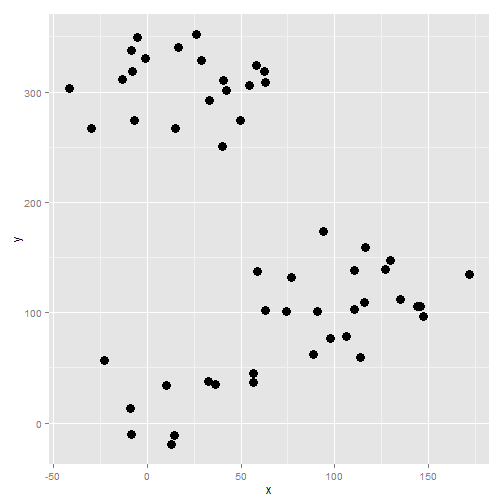
Analysis
Elbow plot
Our main inspiration is that post on stackoverflow:
And the help of the Nbclust package.
The first way to determine a reasonnable number of cluster that was taught at school was the elbow plot. The concept is to plot the sum of the distance between the centroid of the cluster and the point of the cluster by cluster.
The plot looks like an elbow and the classic rule is to take the number of cluster where the curve begin to flaten. Afterward, each new cluster is not really separated from the others.
Elbow plot:
wss <- (nrow(mat)-1)*sum(apply(mat[, -3],2,var))
  for (i in 2:15) wss[i] <- sum(kmeans(mat[, -3],
                                       centers=i)$withinss)

wss2 <- data.frame(x = 1:15, wss = wss)

ggplot(data = wss2, aes(x = x, y = wss))+
    geom_point(size = 4) +
  geom_line() +
  scale_x_continuous(breaks = 1:15) +
  ggtitle("Elbow plot")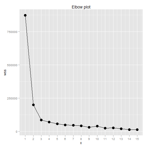
The function NbClust
The function NbClust test a consequent set of methods to determine the optimal number of clusters.
res <- NbClust(mat[, -3], diss=NULL, distance = "euclidean", min.nc=2, max.nc=6,
             method = "kmeans", index = "all")
The different method used (minus the graphical ones) and the number of clusters picked by each:
res$Best.nc## KL CH Hartigan CCC Scott Marriot
## Number_clusters 4.0000 4.0000 3.0000 4.0000 4.0000 4
## Value_Index 14.2718 177.7792 70.9745 12.8076 63.3226 21533263829
## TrCovW TraceW Friedman Rubin Cindex DB
## Number_clusters 3 4.0 4.0000 4.0000 2.0000 2.0000
## Value_Index 865542437 100208.3 29.1325 -15.5892 0.3378 0.4902
## Silhouette Duda PseudoT2 Beale Ratkowsky Ball
## Number_clusters 2.0000 2.0000 2.0000 2.0000 2.0000 4.00
## Value_Index 0.6801 0.5541 15.2897 0.7645 0.5266 43015.13
## PtBiserial Frey McClain Dunn Hubert SDindex Dindex SDbw
## Number_clusters 2.0000 1 2.0000 2.0000 0 2.0000 0 2.000
## Value_Index 0.8523 NA 0.3164 0.4025 0 0.0156 0 0.173Most common value:(Without 0)
summary(res$Best.nc[1,][res$Best.nc[1,]!= 0])## Min. 1st Qu. Median Mean 3rd Qu. Max.
## 1.000 2.000 2.000 2.792 4.000 4.000In the end, the median of all these methods is choosed. In this case, 2.
Result
The plot:
mat$res <- res$Best.partition

ggplot(data = mat, aes(x = x, y = y, colour = factor(res))) +
    geom_point( size = 4)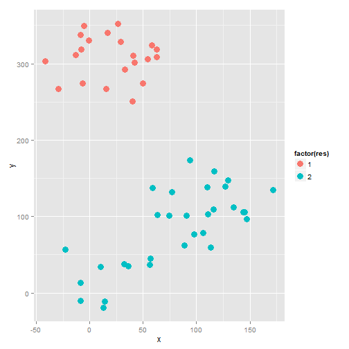
There is another approach we didn’t had time to look at, but which seems promising: The package BHC which does bayesian hierarchical clustering could also provide us an insight on the best cluster.


Leave a Comment